Data Rates are Dead

With the introduction of 802.11ax and its hundreds of new data rates, it’s time to start looking at the MCS Index to better understand link quality. Data rates are now too easy to misinterpret, particularly if, like me, you first learned about Wi-Fi in the days when the number of available data rates was small enough to memorize. Let me explain some of the reasons why.

In Wi-Fi, a data rate is used to describe the number of bits per second that are possible to transmit across the link given the current modulation, coding, channel width, guard interval, active spatial streams, and now resource unit allocation. Data rates are marked in each frame, which allows us to understand how slow or fast each frame was transmitted. We also use data rates to estimate the real throughput that is achievable at the upper layers, with a rough rule of thumb that throughput is roughly 40-60% of the Wi-Fi data rate. That’s because the 802.11 protocol has a lot of overhead which uses up some of the bits that are transmitted across the link, and because of its contention mechanism, which prevents data transfer while channel access is achieved. This is true even in a WLAN with a single access point and a single client.

I will explain what a data rate really means and make the case that the MCS Index actually is much more useful and straightforward. Not just because MCS is a simple scale of whole numbers, but because it tells us more important and direct information about the link quality.

The first problem with data rates is that they can be easily misinterpreted, even when we understand the limitations of the protocol I outlined above. It is very tempting to interpret an 802.11 data rate the way we interpret an 802.3 data rate (Ethernet speed)–it’s the “speed” of the link. The first problem with that idea is that 802.11 data rates are very dynamic, frequently changing to account for changing RF conditions and differing data rate requirements for each frame type. The other problem is that 802.11 has a contention problem that today’s Ethernet doesn’t have to deal with in switched networks.

For example, we understand that if there are many Wi-Fi stations actively using a channel, each station’s application throughput will be greatly reduced even though each station may maintain its highest possible data rate, because the channel is a shared medium. The data rate of the frames is very high, but the rate at which frames are transmitted has dropped for each station. Because of that we should understand that each station’s real bit rate will also be greatly reduced (not the data rate). That is to say, despite maintaining high 802.11 data rates, if we are counting the bits that are transmitted over time, we will find a bits per second value that is much lower than the data rate of each frame in that scenario.

The 802.11 data rate is a result of this calculation:

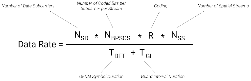
A data rate really only tells us about the speed of a single frame, and doesn’t factor in time lost to contention, lost frames that must be retransmitted, RTS/CTS overhead, efficiency gained from aggregation, etc. It is only relevant to the single frame it is calculated against, not the overall bit rate that is achieved over a period of time.

Of course many wireless engineers already understand this, but can still fall into a trap when interpreting 802.11 data rates. A data rate can mislead us about what to expect from the real flow of frames carrying application traffic. The word “rate,” expressed in “bits per second” can trick us into believing it is telling us something more about the overall speed of all of the frames transmitted across the link, in the same way that an 802.3 data rate tells us about speed in Ethernet. All we really know in Wi-Fi is that the data rate is the speed of just one frame.

So what good is knowing a station is operating at an 866 Mbps data rate, if that really doesn’t tell us what its real bit rate is, let alone the throughput achieved at the higher layers?

What I prefer over 802.11 data rates, which now number in the hundreds with 802.11ax, is the simple MCS Index. Despite appearing abstract at first glance, it actually tells us something much more useful and direct than data rates: It tells us the modulation in use, which the station has chosen in response to current channel conditions. It is true that BPSK, QPSK, 16-QAM, 64-QAM, 256-QAM, and now 1024-QAM are not the easiest things to understand. But spend 10 minutes with Keith Parsons and you are well on your way.

The MCS Index is a simple whole number scale that ranges from 0 all the way up to 11 for 802.11ax stations. It is shorthand for the modulation and coding scheme used, regardless of spatial streams, guard interval, channel width, and now OFDMA resource unit allocation.

Just as data rates really only tell us about a single frame, the same is true for the MCS Index. It changes in tandem with data rates. But it doesn’t come with the same cognitive baggage that data rates do. We know frames are modulated differently for many reasons. We also know that we usually want that modulation to be higher than lower, to improve the efficiency and speed of the link. But we don’t look at the MCS Index and fool ourselves into believing there is a certain number of bits per second achievable for each value on the table. Well, as long as we don’t look over at the corresponding data rates and fall into the old trap again!

Another point in favor of the MCS Index is that we don’t misjudge link quality based on a data rate, both on the high side and low side of the available data rate table. Here’s an example with 802.11ax stations:

MCS	Modulation	Coding	STA 1	STA 2	STA 3
0	BPSK	1/2	8.6 Mbps	34.4 Mbps	0.9 Mbps

All of these data rates use the same modulation (BPSK) and coding (1/2). These are the lowest data rates that an 802.11ax station might shift to depending on its capabilities, rate shifting algorithm, and RU allocation in OFDMA. Why are they so different? Because…

STA 1 is a 1 spatial stream station, using 20 MHz channel width
STA 2 is a 2 spatial stream station, using 40 MHz channel width
STA 3 is a 1 spatial stream station, using a 26 tone OFDMA RU

It is a mistake to believe that STA 2 in this example could support ~ 20 Mbps of application throughput, and it is another mistake to believe that STA 2 is likely experiencing significantly better channel conditions than the other stations that allow it to use a higher data rate. In reality, STA 2, just like the other two, has shifted to the lowest data rate is has available to try to punch through a really challenging RF environment. And despite the higher data rate, the real achievable application throughput for STA 2 may be less than 1 Mbps. In practice, throughput will occasionally be zero during periods when none of its frames are successfully received at the other end of the link. The old throughput rule of thumb falls apart at the bottom of the scale.

What the MCS Index tells us is much more important: Each of these stations is using its most robust and slowest modulation and coding (BPSK and 1/2 coding, or MCS 0) because the channel conditions are terrible, and that’s the real problem. It’s better to set aside flawed throughput estimates and old data rate assumptions and focus on the RF. When we fix that, we know that application performance will be restored. MCS 0 is a warning sign for all stations regardless of their capabilities and operating modes. The only difference that may need to be considered is that equivalent MCS values need 3 dB more of SNR each time the channel width doubles.

Now, when RF conditions on the channel are improved the data rates for the same STA’s might look like this:

MCS	Modulation	Coding	STA 1	STA 2	STA 3
11	1024-QAM	5/6	143.4 Mbps	573.5 Mbps	14.7 Mbps

If we interpret the data rates the old way, it appears that STA 3 might be having trouble compared to STA 1 and especially STA 2, when in reality they are all using the same modulation and coding, 1024-QAM and 5/6 coding, represented as MCS 11. Each station has determined that the channel conditions are so good they can use their most delicate and fastest modulation, 1024-QAM. That’s all we really need to know. The resulting data rates that factor channel width, GI, spatial streams, SU/MU operation, and scheduled RU allocation obfuscate that valuable insight.

That problem has gotten much worse with 802.11ax and its incredible range in data rate values that correspond to the same MCS value. Just within MCS 11, 802.11ax data rates range from 12.5 Mbps to 2402 Mbps, and that assumes no more than 2 spatial streams! It’s no longer possible to look at data rates and understand the quality of the wireless link like we used to. We must start using MCS for that.

It is true that the maximum data rate a STA can achieve does tell us something about the absolute maximum application throughput that it is capable of, so during WLAN design we should consider that if we get the chance to influence client selection, in order to make sure they can fulfill the application requirements we must meet. But more often our goal is simply to get the best wireless performance possible from each station, regardless of their capabilities, not setup a Wi-Fi drag race.

For these reasons I prefer to use the MCS Index over data rates. To interpret it, we only need to understand that each PHY has a different maximum MCS Index value (MCS 7 for 802.11n with 1 spatial stream, MCS 9 for 802.11ac, and MCS 11 for 802.11ax), and wider channel widths require a bit more SNR.